Attention Layer Explained with Examples

Geoffrey Hinton mentioned his concern about back-propagation used in neural networks once in an interview, namely it is used too much. On the other side, he stated a fact about neural networks: they are just stacked nonlinear math functions, and the only requirement for those functions: 1st-order differentiable on either side (left/right).

• All activation functions, Sigmoid, Tanh, RELU and their variant meet the requirement.
• A Convolutional Layer can actually be formulated as a matrix multiplication (see here), which is no difference with a fully connected linear layer.
• A Recurrent Layer reuses its previous results, but still differentiable.
• A Latent Layer is modeled by hyper-parameters, which are deterministic differentiable.

Reference(s):
Draw: A Recurrent Neural Network For Image Generation (arXiv:1502.04623)

Check out code here.

In the paper the attention mechanism is explained as the foveation of the human eye. In a more technical sense, the trick is to use differentiable functions to extract a patch of data. For a time series, the extracted data is a small sequence. For a 2D image, it is a small patch from the original image, rescaled to a fixed size. The patch size in original data is not fixed, but the patch size after extraction is fixed.

Why don’t we just crop the raw data directly and rescale it? To crop, we have to choose an integer for the crop dimension. Whatever function we use to generate the integer, it cannot be a differentiable function.

If there is a way to do the crop + rescale with 1st-order differentiable functions, we can use backpropagation to train the parameters in the function. The solution is to use filter functions.

Filter function

No signal processing, no convolution. Here we filter a function simply by the element-wise multiplication. In the figure below, the top row is a sequence along x. To extract data, the first row is multiplied by placing the filter (second row) at that location. We end up with data in the third row. These filter functions can also be thought as smoothing/blurring functions. In image processing, gaussian is preferred due to its smoothness (see Gaussian blur here).

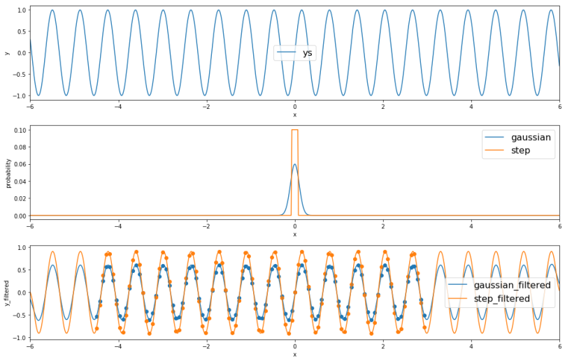
Figure: The top row are raw data (sine wave), the middle row are filter functions (gaussian and step function), and the bottom row are filtered data.

Some technical details: Data dimension N=800, Filter dimension M = 800. How to crop raw data, e.g. from ys[100:600] to a new vector of dimension L = 100? (Btw, the rescale is done automatically.)
- Use L=100 gaussian filters equally placed between [100:600]
Here we can use either gaussian or step function. The end results are the orange and blue dots in the previous figure. (downsampling + low pass filter) The process can be expressed as a matrix product. , where Y is crop and rescaled data, X is raw data. For K, its 100 rows are filters we talked above. Clearly no matter what range of X is ([100:600] or [100:300]), it can always be transformed to Y with a fixed dimension [100].

Only matrix multiplications are used, thus the functions are differentiable. Here is a summary of parameters needed for the process.

• x, center of raw data, e.g. center of [100:600] (also called center of attention)
• and for all (e.g. 100) gaussian distribution

Those parameters are outputs from neural networks.Then, with these parameters, we generate inputs for neural networks. Let’s call this layer a 1D attention layer.

2D Attention Layer

No, we are not going to use bivariate gaussian filters. (Most likely for memory saving. Also the actual weighting is a bit different with 1D gaussians.) Instead, we first look at the data as a mini-batch of rows and we use a 1D attention layer to process them. The processed result is then taken as a mini-batch of columns and we use another 1D attention layer .
A summary of parameters:

• gx,  gy: center of attention
• and : two stacks of 1D attention layers
• : stride, distance between equally spaced gaussian filters
• : use to scale final output

Let’s look at how this attention model works in codes. is not used here.

from scipy.misc import logsumexp

# plot original image
plt.imshow(img, cmap='gray')

# apply 2D attention; play with parameters below
gx, gy = 200, 200
delta = 10
A, B = img.shape
N = 25
mu_x = gx + (np.arange(A)-N//2-0.5)*delta
mu_y = gy + (np.arange(B)-N//2-0.5)*delta
sigma = 1
Fx = np.zeros((N, A))
Fy = np.zeros((N, B))

for i in range(N):
    for a in range(A):
        Fx[i,a] = -(a-mu_x[i])**2/2/sigma**2
    Fx[i,:] = np.exp(Fx[i,:]-logsumexp(Fx[i,:]))

for j in range(N):
    for b in range(B):
        Fy[j,b] = -(b-mu_y[j])**2/2/sigma**2
    Fy[j,:] = np.exp(Fy[j,:]-logsumexp(Fy[j,:]))

filtered_img = Fx.dot(img).dot(Fy.transpose())

plt.figure(figsize=[8,8])
plt.imshow(filtered_img, cmap='gray')

 

Figure: Left is the original image, right is extracted with the attention trick.

In the figure above, the right is extracted from the original image, so the rest of the image is invisible to following layers. Image blurring is controlled by , which is used in the gaussian filters. The stride controls how far apart gaussian filters are. The further apart filters are, the bigger the patches is in the original image.

Next, let’s tune these parameters to see their effects.

1.
By increasing , we are zooming out the original image. And we can see obvious artifacts when the original image cannot fully fill our attention layer image.

Figure: Increase

2.
Increasing makes the image more blurry.

Figure: Increase

3. gx and gy
Changing gx, and gy only shifts the original image. (It’s shifting downward with gx, because of the coordination convention used in image processing.) Also, when we ran out of the original image, we see an elongated neck.

Figure: Increase gx

4.
It is not included in this test, but it just scales the final output linearly.

At last, let’s have a look at the reverse transform in the figure below: from an attention image to an output image. The image is more blurry, and the rest of the image is filled with black. This reverse process is possible because and .

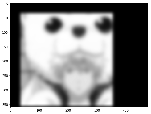
Figure: A transformed image from an attention layer

Conclusion

Attention layer is namely a fancy way to crop (and restore later) part of an image, which is still differentiable and thus compatible with back-propagation.